

If you have ever pushed a spreadsheet past its breaking point — nesting formulas until the cell reads like a short story — Mathematica occupies the territory on the other side of that wall. It is a notebook environment where equations are not just calculated but manipulated symbolically, where a plot is a line of code and a sentence in plain English can summon a model.
What stayed familiar in the current release?
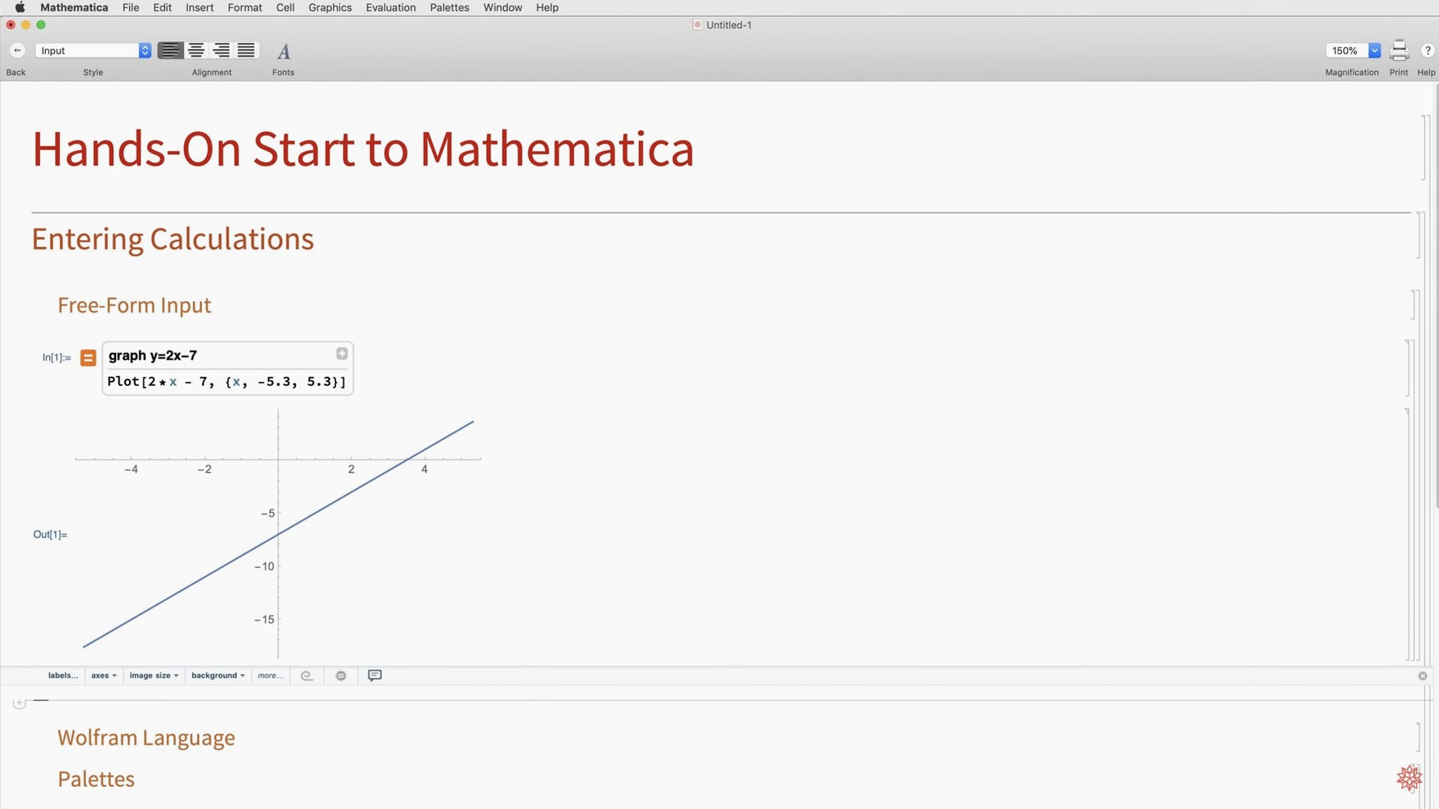
The notebook interface remains the central metaphor, mixing text, live code and rendered output in a single scrolling document. Apple Silicon and Intel Macs are both supported, and the natural-language input — type a question, get a result — still lowers the entry barrier for people who think in sentences rather than syntax.
What new mathematics arrived?
Version 14.3 brings Hilbert transforms and Lommel functions into the symbolic toolkit, alongside new matrix decompositions. On the geometry side, geodesic computation now handles distances along curved surfaces natively.
How did visualization change?
ListFitPlot joins the plotting family, surface plotting functions have been expanded, and vector-based maps offer crisper geographic output. Mesh processing tools round out the set, making it easier to refine 3D geometry before rendering.
What about the tools around the math?
Python and R integration is noticeably faster, LLMGraph taps into large language models for graph construction, and ColumnwiseCombine streamlines data wrangling. System model validation tools and Markdown export support make the workflow feel less bound to the notebook itself.
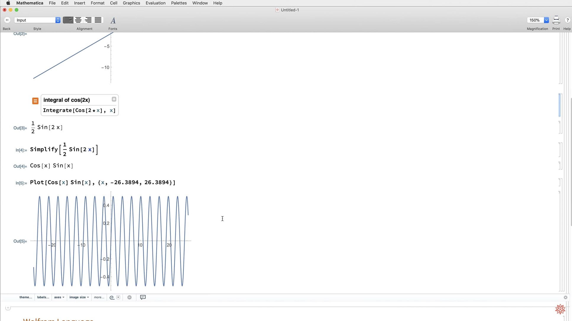
There is a quiet satisfaction in watching a differential equation resolve into a closed form without a single floating-point compromise. The symbolic engine remains the core of Mathematica, and starting a session by declaring assumptions up front — $Assumptions = {t > 0, Element[n, Integers]} — saves a surprising amount of backtracking later. When a calculation stalls, the culprit is often a lingering numeric definition from an earlier cell; clearing the global context with Clear["Global`*"] before a new problem is a ritual worth adopting early.
Solving a parameter sweep from start to finish
Imagine you need to understand how the period of a nonlinear pendulum depends on its initial angle. The textbook small-angle approximation gives you a neat formula, but you want the real curve, and you want it visualised before lunch.
Open a fresh notebook and set the scene by defining the exact period integral. Type the symbolic expression directly, then wrap it in NIntegrate inside a Table that walks the initial angle from five degrees to eighty in steps of two. Mathematica will crunch through the elliptic integrals without complaint, returning a list of pairs almost before your finger lifts from the return key.
The natural next move is ListPlot, but the new ListFitPlot is better here. Feed it the same list and it overlays a fitted curve automatically, giving you a smooth read on where the period begins to climb steeply. Add a second dataset — the small-angle approximation as a flat reference line — and the comparison is immediate. Before you export, switch the notebook colour theme in Preferences to the new dark mode palette; the vector-based plot redraws with adjusted contrast that holds together on a projector. Export the graphic as a high-resolution PDF, copy the notebook cell with the fitted equation into a Markdown cell, and save the whole document as a self-contained report using the new Markdown export. One notebook, one problem, done.
Treat it like a document, not a one-line calculator
The most common stumble is treating Mathematica like a calculator with a big screen. Users type a single expression, evaluate it, and then type another, building up a loose sequence of disconnected outputs. The notebook rewards a different rhythm — defining functions early, reusing them, and letting the symbolic layer do the bookkeeping. Without that shift, you end up copying and pasting numbers by hand, which defeats the point.
Another frequent trap involves delayed versus immediate assignment. Writing f[x] = RandomReal[] freezes a single random value at definition time, while f[x_] := RandomReal[] rolls fresh each call. The underscore and colon look like typographic noise to a newcomer, but they control whether your Monte Carlo simulation actually simulates anything. Related to this: forgetting that Mathematica keeps everything in memory until you quit. A dozen large datasets and a few high-resolution plots can quietly consume gigabytes. Using MemoryInUse[] now and then builds awareness of what your notebook is actually holding.
Finally, beginners often ignore the documentation centre built into the application. The help browser is not a dry manual; every function page includes live examples you can edit and evaluate in place. Spending ten minutes with the tutorial for a single plotting function teaches more idioms than a week of guessing syntax from web searches.
Symbolic expressions versus numeric arrays at the core
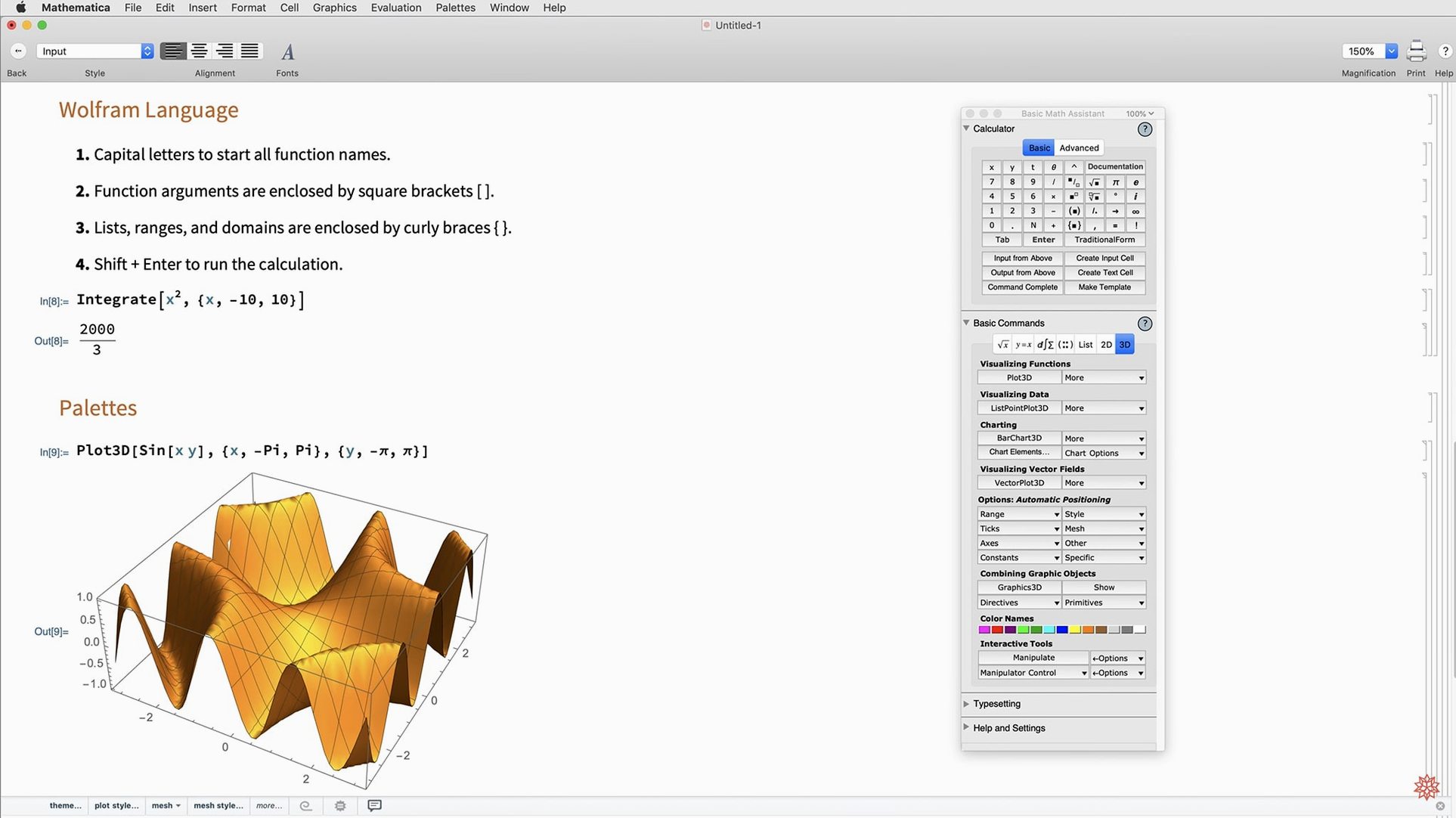
MATLAB and Mathematica both handle matrices and data visualisation, but they part ways at the philosophical level. MATLAB thinks in arrays; everything is a matrix, and the language is procedural at heart. Mathematica thinks in expressions. A polynomial, a graphic, a sound sample — they are all symbolic objects you can pass around, transform, and nest. If your work centres on control systems or large-scale numerical linear algebra, MATLAB’s toolboxes are hard to beat. If you need to solve integrals analytically while rendering the result as an interactive 3D figure, Mathematica is the native habitat.
Maple shares the symbolic ambition but feels more like a reference library than a unified environment. Its typesetting is excellent, and certain differential equation solvers are genuinely deep, yet the notebook front end and the programming language sit less comfortably together. Moving from a derived result to a deployable interactive dashboard is straightforward in Mathematica — a few Manipulate commands and you are done — while in Maple the path is less direct.
On the open-source side, Jupyter with a SymPy kernel covers basic symbolic work and costs nothing, which makes it appealing for a student notebook. The gap appears when the problem scales. SymPy struggles on integrals that Mathematica dispatches in a second, and the plotting tools demand considerably more scaffolding. JupyterLab plus Python is a fine general-purpose stack, but it is an assembly of pieces rather than a single coherent design.
Tune the dark-mode palette before your first notebook
Begin by tuning the interface to match your working hours. Under Preferences, switch the appearance to match the system setting so the new dark mode activates automatically in the evening. The new standard colours for light and dark environments mean plots will not blind you during a late session, and the notebook background shifts without you needing to touch a stylesheet.
On day one, type a few sentences in natural language just to see what the parser understands. Something like “plot the Bessel function of the first kind for orders 0 through 4” gives you a working visualisation and, crucially, the underlying Wolfram Language code that produced it. Reading that generated code is a shortcut to learning the syntax faster than any textbook introduction.
Spend an hour with the new LLMGraph function if language models interest you. Feed it a paragraph of text — a news summary or a poem — and it constructs a graph of entities and relationships you can manipulate with the rest of the system. The integration feels experimental in the best way, like a door propped open toward a different kind of computation.
Set a habit of saving notebooks frequently in the native format but also exporting key results through the new Markdown path. Having a clean text version of your derivations, equations and all, makes them searchable outside the application and easier to share with collaborators who do not have Mathematica installed. Finally, bookmark the ListFitPlot and geodesic computation documentation pages. They are small additions to the function library, but they will surface in your workflows more often than you expect once you know they are there.
Version 14.3 introduces full dark-mode support alongside new standard colours tuned for both light and dark environments. The mathematics engine gains Hilbert transforms, Lommel functions and additional matrix decompositions. Visualization expands with ListFitPlot, enhanced surface plotting, vector-based maps and mesh processing tools. Beyond the core, geodesic computation, LLMGraph, faster Python and R integration, ColumnwiseCombine, system model validation tools and Markdown export all ship in this release.
- macOS 12 or later
- Apple Silicon or Intel 64-bit processor
Questions from the booth
Yes, version 14.3 runs natively on both Apple Silicon and Intel 64-bit Macs running macOS 12 or later.